Emulation Control Design

Assuming that $C(s)$ only has simple poles…
$C(s)={\sum }_{i=0}^n\frac{c_i}{s-p_i}=[1\dots 1]\left[\begin{array}{ccccc}\frac{1}{s-p_1}& & & & \\ & & \dots & & \\ & & & & \frac{1}{s-p_n}\end{array}\right]\left[\begin{array}{c}{c}_1\\ \dots \\ c_n\end{array}\right]$
Which comes in our form $C(s)=C(sI-A{)}^{-}1B$ from our State Space Models.

If we call
$\dot{x}=\left[\begin{array}{ccccc}{p}_1& & & & \\ & & \dots & & \\ & & & & p_n\end{array}\right]x+\left[\begin{array}{c}{c}_1\\ \dots \\ c_n\end{array}\right]e$ which is of the form $\dot{x}=Ax+Be$
and $u=[1\dots 1]x=Cx$

We can now put this into $x^{+}=\hat{A}+\hat{B}e$ form

Hint

As a reminder, our goal is to approximate our continuous controllers by emulating them with discrete controllers. Here is how we do that.

From CT to DT

Applying the left side rule from Integration Approximation Techniques

$\Delta [k+1]=T(Ax(kT)+Be(kT))=T(Ax[k]+Be[k])$
$x[k+1]=x[k]+T(Ax[k]+Be[k])$

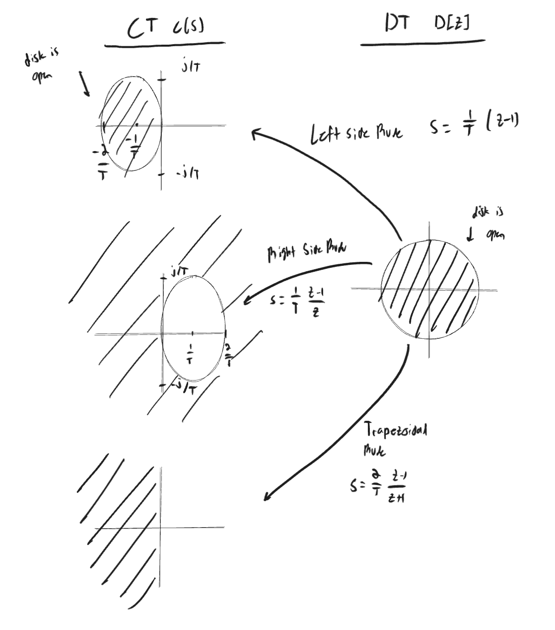
Taking a z-transform…
$zX[z]=X[z]+T(AX[z]+BE[z])⟹((z-1)I-TA)X[z]=TBE[z]⟹X[z]=((z-1)I-TA{)}^{-1}TBE[z]$ $⟹X[z]=\left[\begin{array}{ccccc}\frac{1}{z-1-T_{p_1}}& & & & \\ & & \dots & & \\ & & & & \frac{1}{z-1-T_{p_n}}\end{array}\right]\left[\begin{array}{c}Tc1\\ \dots \\ Tcn\end{array}\right]E[z]$
$⟹u(t)=Cx(t)⟹u[k]=Cx[k]⟹U[z]=CX[z]=[1\dots 1]\left[\begin{array}{c}\frac{T{c}_1}{z-1-T{p}_1}\\ \dots \\ \frac{T{c}_n}{z-1-T{p}_n}\end{array}\right]E[z]={\sum }_{i=1}^n\frac{Tci}{z-1-T_{p_i}}E[z]$ $⟹u[z]={\sum }_{i=1}^n\frac{c_i}{\frac{1}{T}(z-1)-p_i}E[z]$ Where the sum in front of $E[z]$ is our Discrete Time controller $D[z]$ $⟹D[z]=C(s){|}_{s=\frac{1}{T}(z-1)}$

Applying the right side rule from Integration Approximation Techniques

$\Delta [k+1]=T(Ax[k+1])+Be[[k+1])$
$x[k+1]=x[k]+T(Ax[k+1]+Be[k+1])$

Taking a z-transform…
$zX[z]=X[z]+T(AzX[z]+BzE[z])⟹((z)I-TA)X[z]=TBzE[z]⟹X[z]=(z(I-TA)-I{)}^{-1}TBzE[z]$ $⟹X[z]=\left[\begin{array}{ccccc}\frac{1}{z(1-T_{p_1)}-1}& & & & \\ & & \dots & & \\ & & & & \frac{1}{z(1-T_{p_n})-1}\end{array}\right]\left[\begin{array}{c}Tz{c}_1\\ \dots \\ Tz{c}_n\end{array}\right]E[z]$
$⟹u[z]=Cx[z]=[1\dots 1]\left[\begin{array}{c}\frac{Tz{c}_1}{z(1-T{p}_1)-1}\\ \dots \\ \frac{Tz{c}_n}{z(1-T{p}_n)-1}\end{array}\right]E[z]={\sum }_{i=1}^n\frac{Tz{c}_i}{z(1-T_{p_i})-1}E[z]={\sum }_{i=1}^n\frac{c_i}{\frac{1}{T}\left(1-\frac{1}{z}\right)-p_i}E[z]$
$⟹D[z]=C(s){|}_{s=\frac{1}{T}(1-\frac{1}{z})}$

Applying the Trapezoidal rule from Integration Approximation Techniques

$\Delta [k+1]=\frac{T}{2}(Ax[k]+Be[k]+Ax[k+1]+Be[k+1])$
$x[k+1]=x[k]+\Delta [k+1]=x[k]+\frac{T}{2}(Ax[k]+Be[k]+Ax[k+1]+Be[k+1])$

Taking a z-transform…
$zX[z]=X[z]+\frac{T}{2}(AX[z]+BE[z]+AzX[z]+BzE[z])$
$\left(z\left(I-\frac{T}{2}A\right)-\left(I+\frac{T}{2}A\right)\right)X[z]=\frac{T}{2}B(z+1)E[z]$
$X[z]={\left(z\left(I-\frac{T}{2}A\right)-\left(I+\frac{T}{2}A\right)\right)}^{-1}\frac{T}{2}B(z+1)E[z]$

$X[z]⟹\left[\begin{array}{ccccc}z\left(1-\frac{T}{2}{p}_1\right)-\left(1+\frac{T}{2}A\right)& & & & \\ & & \dots & & \\ & & & & z\left(1-\frac{T}{2}{p}_n\right)-\left(1+\frac{T}{2}{p}_n\right)\end{array}\right]\left[\begin{array}{c}\frac{T}{2}(z+1)c_1\\ \dots \\ \frac{T}{2}(z+1)c_n\end{array}\right]E[z]$
$=\left[\begin{array}{c}\frac{\frac{T}{2}(z+1)c_1}{z\left(1-\frac{T}{2}{p}_1-\left(1+\frac{T}{2}{p}_1\right)\right)}\\ \dots \\ \frac{\frac{T}{2}(z+1)c_n}{z\left(1-\frac{T}{2}{p}_n-\left(1+\frac{T}{2}{p}_n\right)\right)}\end{array}\right]E[z]$

$⟹u[z]=Cx[z]=[1\dots 1]\left[\begin{array}{c}\dots \end{array}\right]E[z]={\sum }_{i=1}^n\frac{\frac{T}{2}(z+1)c_i}{z(1-T_{p_i})-1}E[z]={\sum }_{i=1}^n\frac{c_i}{z\left(1-\frac{T}{2}{p}_i\right)-\left(1+\frac{T}{2}{p}_i\right)}E[z]={\sum }_{i=1}^n\frac{c_i}{\frac{2}{t}\frac{z-1}{z+1}-p_i}E[z]$ $D[z]=C(s){|}_{s=\frac{2}{T}\frac{z-1}{z+1}}$

Summary

The sum terms in each one of these u[z] expressions is our D[z] controller

[Excalidraw](Drawing 2025-11-03 11.55.56.excalidraw)

Issues

Left side rule

• All of our poles are in the left-half plane but, we could have poles that are stable in continuous time that are in the left-half plane, that map to unstable poles in discrete time Right side rule
• We recover the entire left-half plane but, we could have poles that are unstable in continuous time that are in the right half plane, that map to stable poles in discrete time Trapezoidal rule
• Stable poles in continuous time iff we have stable poles in discrete time which is out goal

An alternative approximation is…

• Step Invariant Approximation