Simple Pole Approximation

Uses Input-Output Parameterization

Choose poles $\{p_i{\}}_{i=1}^m$ as a part of our control design. We approximate $W\left[z\right]={\sum }_{i=1}^m\frac{w_i}{z-p_i}$ where $w_i\in \mathbb{C}\forall i$

Warning

When you choose $m$, you need to choose $m\ge 2\times \text{ \#unstable plant poles}$

Note

You can use poles of multiplicity 1 (simple poles) to approximate infinite poles pretty well

Assume plant $G[z]={\sum }_{k=1}^n\frac{c_k}{z-q_k}$ where $\{q_k{\}}_{k=1}^n$ are the plant poles.
Assumption $G[z]$ has only simple poles.

We can split these poles in stable and unstable components:
Stable: \lbrace{q_{k}}\rbrace^\hat{n}_{k=1} and Unstable: \lbrace{q_{k}}\rbrace^\hat{n}_{k=\hat{n}+1}

Final Result

• $\alpha =\frac{c_k}{p_i-q_k}$
• $\beta =\frac{c_k}{q_k-p_i}$
• $\gamma =\frac{c_j}{q_j-p_i}$
• ${\hat{\gamma }}_{j,k}=\frac{c_j}{q_j-q_k}$
• $G\left[z\right]W\left[z\right]={\sum }_{k=1}^n\left({\sum }_{i=1}^m{\beta }_{ki}{w}_i\right)\frac{1}{z-q_k}+{\sum }_{i=1}^m{\alpha }_i{w}_i\frac{1}{z-p_i}$
• $X\left[z\right]=1+{\sum }_{k=1}^{\hat{n}}\frac{{\hat{x}}_k}{z-q_k}+{\sum }_{i=1}^m\frac{x_i}{z-p_i}$
• Where after comparing coefficients we can conclude…
  • Eqn’ 1:
  • ${\hat{x}}_k=-{\beta }_{ki}{w}_i\forall k\in \left\{1,\dots ,\hat{n}\right\}$
  • $x_i=-{\alpha }_i{w}_i\forall i\in \left\{1,\dots ,m\right\}$
  • $0={\sum }_{i=1}^m-{\beta }_{k,i}{w}_i\forall k\in \hat{n}+1,\dots ,n$
  • Eqn’ 2
  • $0=-c_j+{\sum }_{i=1}^m-{\gamma }_{j,i}{x}_i+{\sum }_{k=1}^{\hat{n}}-\widehat{{\gamma }_{j,k}}\widehat{x_k}$ (Constraint that V is stable)
  • These ‘-’s appear due to the IOP equation $X[z]=1-G[z]W[z]$

Note on sums and hats and poles and shit

• $n$ is the total number of simple poles in $G[z]$ (before adding an explicit pole)
• $n+1$ is the total number of poles in $G[z]$ after adding explicit poles to a partial fractional expantion
• $\hat{n}$ is the number of distinct stable simple poles $q_k$ that appear in the partial fractional expansion of $X[z]$, typicall this is $\hat{n}=n-\text{unstable poles}$
• $k=\hat{n}+1,\dots ,n+1$ which is the poles whose contributions must cancel

Transient Specs

Informed by Input-Output Parameterization with a Simple Pole Approximation. We use these specs to design a controller.

1. Closed-loop stability ⇐> $W$, $X$, $V$ stable ⇒ already guaranteed by choosing ${p_i}_{i=1}^m\in \mathbb{D}$ and satisfying Eqn’s i and ii
2. $e_{ss}=T_{re}\left[1\right]$ = $X[1]$ [by the IOP theorem part b)] = $1+{\sum }_{i=1}^m\frac{x_i}{1-p_i}+{\sum }_{k=1}^{\hat{n}}\frac{\widehat{x_k}}{1-q_k}$

Case 1.
$e_{ss}=0$
$e_{ss}=1+{\sum }_{i=1}^m\frac{x_i}{1-p_i}+{\sum }_{k=1}^{\hat{n}}\frac{\widehat{x_k}}{1-q_k}=0$ Sometimes we don’t want this to be 0, for example if we have an integrator in our systen

Case 2.
$\left|e_{ss}\right|\le C$
$e_{ss}\le C\text{ \& }{e}_{ss}\ge -C$

3. Limits on the control effort $u\left[k\right]\le C\forall k\ge 0$ → step($T_{ru}$)[k] ≤ C $\forall$ k ≥ 0
   1. Step response of a simple pole: $y\left[k\right]=\frac{1}{1-p}\left(1-p\cdot p^{k-1}\right)=\frac{1-p^k}{1-p}$
   2. $T_{ru}=W$ and needs to be bounded by IOP theorem b
   3. ${\sum }_{i=1}^m\frac{1-p_i^k}{1-p_i}{w}_i\le C\forall k\ge 0$
4. Overshoot $\%O.S\le C$
   1. $y=r-e$ ⇒ $Y=R-E=R-T_{re}R$ assuming disturbance (d) = 0 where $Y=\left(1-T_{re}\right)R=T_{ry}R$
   2. step($T_{ry}$) [ j ] ≤ $(1+C)y_{ss}$ Where we can sub our $T_{ry}$ and $y_{ss}$
   3. step($1-X$)[ j ] ≤ $\left(1+C\right)\left(1-X\left[1\right]\right)$
   4. $$\begin{gathered} \max \left(-{\sum }_{i=1}^m\frac{1-p_i^j}{1-p_i}{x}_i- \\ su{m}_{k=1}^{\hat{n}}\frac{1-q_k^j}{1-q_k}{\hat{x}}_k\right)\le (1+C)(-{\sum }_{i=1}^m\frac{x_i}{1-p_i}+{\sum }_{k=1}^{\hat{n}}\frac{\widehat{x_k}}{1-q_k}) \end{gathered}$$
      1. The left is the step response of $T_{ry}$ and the right is the steady state value of Y (we can go an amount C over Y at any time)
5. Settling time $T_s\le C$
   1. Let T be the sampling time and let $\hat{j}=\min j,jT\ge C$
   2. Let step($1-X$)[ j ] ≥ $1.02y_{ss}$ and $\le 0.98y_{ss}$
   3. $$\begin{gathered} \max \left(-{\sum }_{i=1}^m\frac{1-p_i^j}{1-p_i}{x}_i- \\ su{m}_{k=1}^{\hat{n}}\frac{1-q_k^j}{1-q_k}{\hat{x}}_k\right)\le 1.02(-{\sum }_{i=1}^m\frac{x_i}{1-p_i}+{\sum }_{k=1}^{\hat{n}}\frac{\widehat{x_k}}{1-q_k}) \end{gathered}$$
   4. $$\begin{gathered} \min \left(-{\sum }_{i=1}^m\frac{1-p_i^j}{1-p_i}{x}_i- \\ su{m}_{k=1}^{\hat{n}}\frac{1-q_k^j}{1-q_k}{\hat{x}}_k\right)\ge 0.98(-{\sum }_{i=1}^m\frac{x_i}{1-p_i}+{\sum }_{k=1}^{\hat{n}}\frac{\widehat{x_k}}{1-q_k}) \end{gathered}$$

Vector Form

This will make it more efficient for us to work with the equations above (IOP equations and the specs).
We can define the following…

• $w:-\left[\begin{array}{c}{w}_1\\ \dots \\ w_m\end{array}\right]$
• $x:-\left[\begin{array}{c}{x}_1\\ \dots \\ x_m\end{array}\right]$
• $\hat{x}:-\left[\begin{array}{c}\widehat{x_1},\\ \dots \\ \widehat{x_{\hat{n}}}\end{array}\right]$
• $\alpha :=\left[\begin{array}{ccc}{\alpha }_1& \dots & 0\\ \dots & \dots & \dots \\ 0& \dots & {\alpha }_m\end{array}\right]$
• $\beta :=\left[\begin{array}{ccc}{\beta }_1& \dots & {\beta }_{1,m}\\ \dots & \dots & \dots \\ {\beta }_{\hat{n},1}& \dots & {\beta }_{\hat{n},m}\\ \dots & \dots & \dots \\ {\beta }_{n,1}& \dots & {\beta }_{n,m}\end{array}\right]$
• $\gamma :=\left[\begin{array}{ccc}{\gamma }_{\hat{n}+1,1}& \dots & {\gamma }_{\hat{n}+1,m}\\ \dots & \dots & \dots \\ {\gamma }_{n,1}& \dots & {\gamma }_{n,m}\end{array}\right]$
• $\hat{\gamma }:=\left[\begin{array}{ccc}{\hat{\gamma }}_{\hat{n}+1,1}& \dots & {\hat{\gamma }}_{\hat{n}+1,m}\\ \dots & \dots & \dots \\ {\hat{\gamma }}_{n,1}& \dots & {\hat{\gamma }}_{n,m}\end{array}\right]$

Note

Screenshots cause no way am I writing this out

$X$, $\hat{X}$ and $w$

• Here the two matrices of beta are the stable and unstable poles
• You can also see a couple blocks that are the identity matrix, as well as zero matrices

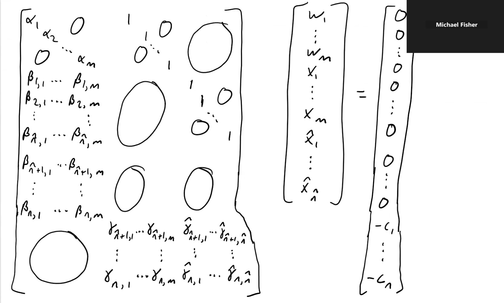
• Here $c$ starts from $c_{\hat{n}+1}$ instead of $c_1$ (typo) We can re-express this larger matrix as…
  $\left[\begin{array}{ccc}\alpha & I& 0\\ \beta & 0& 0\\ 0& \gamma & \hat{\gamma }\end{array}\right]=\left[\begin{array}{c}w\\ x\\ \hat{x}\end{array}\right]=\left[\begin{array}{c}0\\ 0\\ -c_{(}\widehat{n_{+}1:n})\end{array}\right]$
• Let the first matrix = $A$, and the result = $B$

So the IOP eqn’s are:

• $A\left[\begin{array}{c}w\\ x\\ \hat{x}\end{array}\right]=B$

Specifications

• $e_{ss}=1+\left[\frac{1}{1-p_1}\dots \frac{1}{1-p_m}\frac{1}{1-q_1}\dots \frac{1}{1-q_{\hat{n}}}\right]\left[\begin{array}{c}{x}_1\\ \dots \\ x_m\\ \widehat{x_1}\\ \dots \\ \widehat{x_{\hat{n}}}\end{array}\right]\le C$ where $C$ could be $0$
  • This matrix in the middle is the $\text{steady state}$ matrix
• $u[k]\le C$
  • Note: If you don’t reach steady state, choose a larger $k$
  • Fix $k>0$
  • Now we can look at the maximum of $k$ ${\max }_{0<k\le K}{\sum }_{i=1}^m\frac{1-p_i^k}{1-p_i}{w}_i\le C$
  • $u[k]=\left[\begin{array}{ccc}\frac{1-p_1^k}{1-p_1}& \dots & \frac{1-p_m^k}{1-p_m}\end{array}\right]\left[\begin{array}{c}{w}_1\\ \dots \\ w_m\end{array}\right]$
    • The middle TF here is $ste{p}_{ru}$
  • Where each of these partial fractions is $\text{step}{T}_{ru}[1\dots k]$
  • $\max ({\text{step}}_{ru}\ast w)\le C$ where ${\text{step}}_{ru}$ is the matrix of the step response of $T_{ru}[1\dots k]$
• $OS\le C$
  • $\left[\begin{array}{c}step(T_{ry})[1]\\ \dots \\ step(T_{ry})[k]\end{array}\right]=\left[\begin{array}{ccccc}-\frac{1-p_{1^1}}{1-p_1}& \dots & -\frac{1-p_m^1}{1-p_m}-\frac{1-q_1^1}{1-q_1}& \dots & \frac{1-q_{\hat{n}}^1}{1-q_{\hat{n}}}\\ \dots & \dots & \dots & \dots & \dots \\ -\frac{1-p_1^k}{1-p_1}& \dots & -\frac{1-p_m^k}{1-p_m}-\frac{1-q_1^k}{1-q_1}& \dots & \frac{1-q_{\hat{n}}^k}{1-q_{\hat{n}}}\end{array}\right]\left[\begin{array}{c}{x}_1\\ \dots \\ x_m\\ \widehat{x_1}\\ \dots \\ {\hat{x}}_{\hat{n}}\end{array}\right]$
    • Where this middle matrix is $ste{p}_{ry}$
  • $OS=\max (ste{p}_{ry}\left[\begin{array}{c}x\\ \hat{x}\end{array}\right]\le (1+C)(-\text{steady state})\left[\begin{array}{c}x\\ \hat{x}\end{array}\right])$
• $T_s\le C$
  • $ma{x}_{j\ge \hat{j}}(step(T_{ry}[j]))\le 1.02y_{ss}$
  • $mi{n}_{j\ge \hat{j}}(step(T_{ry}[j]))\ge 0.98y_{ss}$
  • Where in matrix notation…
  • $ma{x}_{j\ge \hat{j}}(ste{p}_{ry}[j])\left[\begin{array}{c}x\\ \hat{x}\end{array}\right]\le 1.02y_{ss}(\text{-steady state}\left[\begin{array}{c}x\\ \hat{x}\end{array}\right])$
  • $mi{n}_{j\ge \hat{j}}(stepry[j])\left[\begin{array}{c}x\\ \hat{x}\end{array}\right]\ge 0.98(\text{-steady state}\left[\begin{array}{c}x\\ \hat{x}\end{array}\right])$

Redefinition of Control Design for IOP with SPA

• Given $w$, $x$, $\hat{x}$
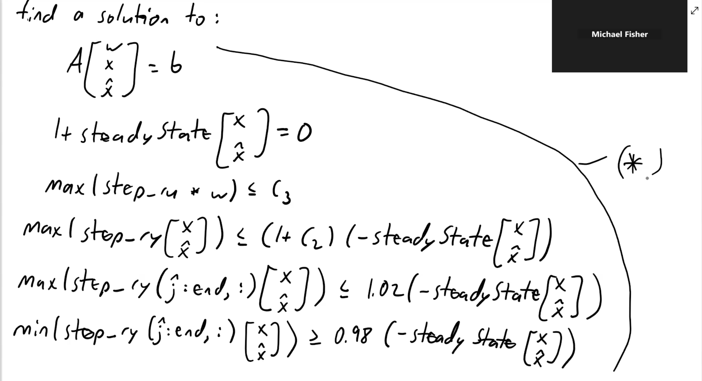
• Find a solution to: $A\left[\begin{array}{c}w\\ x\\ \hat{x}\end{array}\right]=B$
• Where:
  • $e_{ss}=0$
  • $T_s\le C_1$
  • $OS\le C_2$
  • $u[k]\le C_3$
• And these constraints in our matrix form can be viewed from the notation above

We solve this stuff using a numerical solver

Concepts

• Choosing Poles