Finding State Space Realizations

Note

This is a way to represent a transfer function as a set of first-order differential equations in vector form

$\dot{x}=Ax+Bu$ and $y=Cx+Du$…

[Excalidraw for this note](Drawing 2025-10-22 11.38.38.excalidraw)

Rendered image for ssg

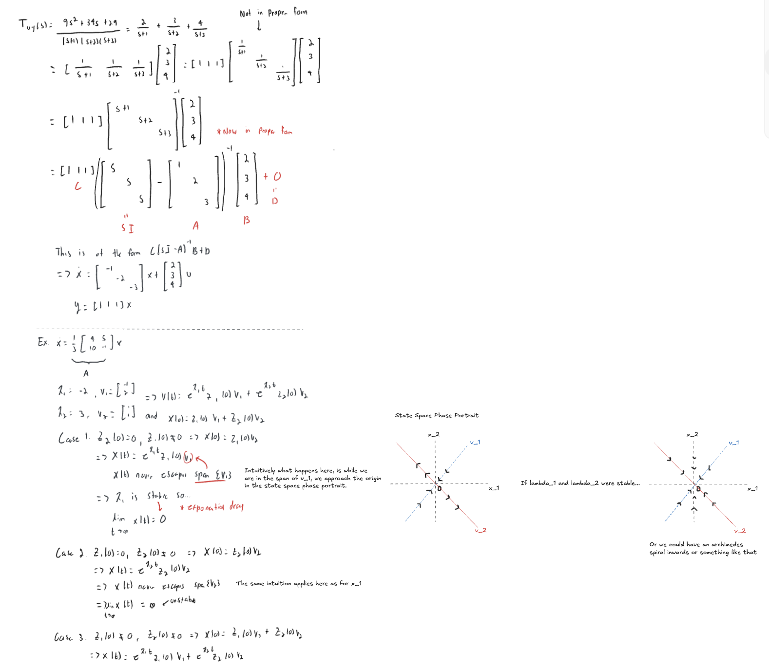
This approach works for any transfer function $T_{uy}(s)$ with only simple poles

Assume $u(t)=0\forall t\ge 0$ and $x^{\prime }=Ax$
Assume A is diagonalizable (sufficient condition: all eigenvalues of A are distinct)
Let ${\lambda }_1,\dots ,{\lambda }_n$ be the eigenvalues of A
Let $v_1,\dots ,v_n$ be their associated eigenvectors (of A)

$\Lambda =\left[\begin{array}{ccccc}{\lambda }_1& & & & \\ & & \dots & & \\ & & & & {\lambda }_n\end{array}\right]$ and $v=\left[\begin{array}{c}{v}_1\dots v_n\end{array}\right]$
$A=V\Lambda V^{-}1$ or $\Lambda =VA{V}^{-}1$

Suppose $x^{\prime }=\left[\begin{array}{c}{x}_1^{\prime }\\ \dots \\ x_n^{\prime }\end{array}\right]\left[\begin{array}{ccccc}{\lambda }_1& & & & \\ & & \dots & & \\ & & & & {\lambda }_n\end{array}\right]\left[\begin{array}{c}{x}_1\\ \dots \\ x_n\end{array}\right]$ where $x^{\prime }=\Lambda x$
Then…
$x_1^{\prime }={\lambda }_1{x}_1$ etc…

Such that:
$x_1(t)=e^{{\lambda }_{1}t}{x}_1(0)$

Note

Note here, each state has dynamics that don’t depend on any other state besides itself. These are decoupled states and dynamics.

Here, we can solve 1st order differential equation rather than an $n^{th}$ order DE since the dynamics are decoupled and we can solve for the dynamics of an isolated state.

Defining a new set of states in a new coordinate system $z=V^{-1}x⟹x=Vz$ and $z^{\prime }=V^{-1}{x}^{\prime }=V^{-1}Ax=V^{-1}V\Lambda V^{-1}x=\Lambda z$
$z^{\prime }=\Lambda z$ showing a decoupled state
$z(t)=e^{{\lambda }_{1}t}{z}_1(0)$ etc…

Then
$x(t)=Vz(t)=\left[\begin{array}{c}{v}_1\dots v_n\end{array}\right]\left[\begin{array}{c}{z}_1(t)\\ \dots \\ z_n(t)\end{array}\right]={\sum }_n^{i=1}{z}_i(t)v_i={\sum }_n^{i=1}{e}^{{\lambda }_{i}t}{z}_i(0)v_i$
What is this intuitively telling us?

Definition

Define an eigenvalue $\lambda (A)$ as stable if $\lambda \in {\mathbb{C}}^{-1}$ and unstable otherwise.

State Space Realization for the DT Feedback System

For $G[z]$ = $x[k+1]=A_{d}x[k]+B_{d}u[k]$ and $y[k]=Cx[k]$
For the plant…

• $D[z]:\hat{x}[k+1]=\hat{A}\hat{x}+\hat{B}(r[k]-y[k])$
• $\bar{u}[k]=\hat{C}\hat{x}[k]+\hat{D}(r[k]-y[k])$
• $u[k]=\bar{u}[k]+d[k]$ Choosing states:
• $\left[\begin{array}{c}x\\ \hat{x}\end{array}\right]$ as a state for the DT feedback system
• $x[k+1]=A_{d}x[k]+B_{d}u[k]=A_{d}x[k]+B_d(\bar{u}[k]+d[k])$
• $=A_{d}x[k]+B_{d}d[k]+B_d(\hat{C}\widehat{x[k]}+\hat{D}(r[k]-y[k]))$ where $y[k]$ here is $Cx[k]$
• We are now expressing $x[k+1]$ in terms of $x[k]$ and the states, eliminating the other input signals
• $=(A_d-B_d\hat{D}C)x[k]+B_d\hat{C}\hat{x}[k]+B_d\hat{D}r[k]+B_{d}d[k]$
• Where we can do the same thing for $\hat{x}$
• $\hat{x}[k+1]=\hat{A}\hat{x}[k]+\hat{B}(r[k]-\hat{B}Cx[k])+\hat{A}\hat{x}[k]+\hat{B}r[k]$